INTRODUCTION
The typical recognition/classification framework in Artificial Vision uses a set of object features for discrimination. Features can be either numerical measures or nominal values. Once obtained, these feature values are used to classify the object. The output of the classification is a label for the object (Mitchell, 1997).
The classifier is usually built from a set of "training" samples. This is a set of examples that comprise feature values and their corresponding labels. Once trained, the classifier can produce labels for new samples that are not in the training set.
Obviously, the extracted features must be discriminative. Finding a good set of features, however, may not be an easy task. Consider for example, the face recognition problem: recognize a person using the image of his/her face. This is currently a hot topic of research within the Artificial Vision community, see the surveys (Chellappa et al, 1995), (Samal & Iyengar, 1992) and (Chellappa & Zhao, 2005). In this problem, the available features are all of the pixels in the image. However, only a number of these pixels are normally useful for discrimination. Some pixels are background, hair, shoulders, etc. Even inside the head zone of the image some pixels are less useful than others. The eye zone, for example, is known to be more informative than the forehead or cheeks (Wallraven et al, 2005). This means that some features (pixels) may actually increase recognition error, for they may confuse the classifier.
Apart from performance, from a computational cost point of view it is desirable to use a minimum number of features. If fed with a large number of features, the classifier will take too long to train or classify.
BACKGROUND
Feature Selection aims at identifying the most informative features. Once we have a measure of " informative-ness" for each feature, a subset of them can be used for classifying. In this case, the features remain the same, only a selection is made. The topic of feature selection has been extensively studied within the Machine Learning community (Duda et al, 2000). Alternatively, in Feature Extraction a new set of features is created from the original set. In both cases the objective is both reducing the number of available features and using the most discriminative ones.
The following sections describe two techniques for Feature Extraction: Principal Component Analysis and Independent Component Analysis. Linear Discriminant Analysis (LDA) is a similar dimensionality reduction technique that will not be covered here for space reasons, we refer the reader to the classical text (Duda et al., 2000).
Figure 1.
As an example problem we will consider face recognition. The face recognition problem is particularly interesting here because of a number of reasons. First, it is a topic of increasingly active research in Artificial Vision, with potential applications in many domains. Second, it has images as input, see Figure 1 from the Yale Face Database (Belhumeur et al, 1997), which means that some kind of feature processing/selection must be done previous to classification.
PRINCIPAL COMPONENT ANALYSIS
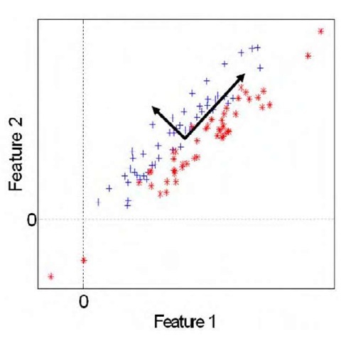
Principal Component Analysis (PCA), see (Turk & Pentland, 1991), is an orthogonal linear transformation of the input feature space. PCA transforms the data to a new coordinate system in which the data variances in the new dimensions is maximized. Figure 2 shows a 2-class set of samples in a 2-feature space. These data have a certain variance along the horizontal and vertical axes. PCA maps the samples to a new orthogonal coordinate system, shown in bold, in which the sample variances are maximized. The new coordinate system is centered on the data mean.
The new set of features (note that the coordinate axes are features) is better from a discrimination point of view, for samples of the two classes can be readily separated. Besides, the PCA transform provides an ordering of features, from the most discriminative (in terms of variance) to the least. This means that we can select and use only a subset ofthem. In the figure above, for example, the coordinate with the largest axis is the most discriminative.
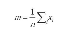
When the input space is an image, as in face recognition, training images are stored in a matrix T Each row of T contains a training image (the image rows are laid consecutively, forming a vector). Thus, each image pixel is considered a feature. Let there be n training images. PCA can then be done in the following steps:
1. Subtract the mean image vector m from T, where:
2. Calculate the covariance matrix C:
3. Perform Singular Value Decomposition over C, which gives an orthogonal transform matrix W
Figure 2.
Figure 3.
4. Choose a set of "eigenfaces" (see below)
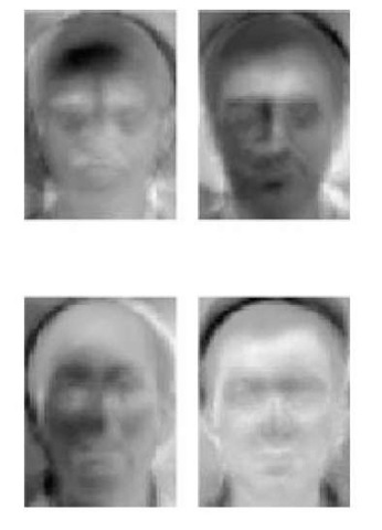
The new feature axes are the columns of W These features can be considered as images (i.e. by arranging each vector as a matrix), and are commonly called basis images or eigenfaces within the face recognition community. The intensity of the pixels of these images represents their weight or contribution in the axis. Figure 3 shows the typical aspect of eigenfaces.
Normally, in step 4 above only the best K eigenvectors are selected and used in the classifier. That is achieved by discarding a number of columns in W. Once we have the appropriate transform matrix, any set X of images can be transformed to this new space simply by:
1. Subtract the mean m from the images in X
2. Calculate Y = XW
The transformed image vectors Yare the new feature vectors that the classifier will use for training and/or classifying.
INDEPENDENT COMPONENT ANALYSIS
Independent ComponentAnalysis is a feature extraction technique based in extracting statistically independent variables from a mixture of them (Jutten & Herault, 1991, Comon, 1994). ICA has been successfully applied to many different problems such as MEG and EEG data analysis, blind source separation (i.e. separating mixtures of sound signals simultaneously picked up by several microphones), finding hidden factors in financial data and face recognition, see (Bell & Sejnowski, 1995).
The ICA technique aims at finding a linear transform for the input data so that the transformed data is as statistically independent as possible. Statistical independence implies decorrelation (but note that the opposite is not true). Therefore, ICA can be considered a generalization of PCA.
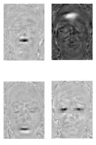
The basis images obtained with ICA are more local than those obtained with PCA, which suggests that they can lead to more precise representations. Figure 4 shows the typical basis images obtained with ICA.
ICA routines are available in a number of different implementations, particularly for Matlab. ICA has a higher computational cost than PCA. FastICA is the most efficient implementation to date, see (Gavert et al, 2005).
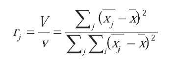
As opposed to PCA, ICA does not provide an intrinsic order for the representation coefficients of the face images, which does not help when extracting a subset of K features. In (Bartlett & Sejnowski, 1997) the best results were obtained with an order based on the ratio of between-class to within-class variance for each coefficient:
Figure 4.
where Vis the variance of the j class mean and v is the sum of the variances within each class.
FUTURE TRENDS
PCA has been shown to be an invaluable tool in Artificial Vision. Since the seminal work of (Turk & Pentland, 1991) PCA-based methods are considered standard baselines in the problem of face recognition. Many other techniques have evolved from it: robust PCA, nonlinear PCA, incremental PCA, kernel PCA, probabilistic PCA, etc.
As mentioned above, ICA can be considered an extension of PCA. Some authors have shown that in certain cases the ICA transformation does not provide performance gain over PCA when a "good" classifier is used (like Support Vector Machines), see (Deniz et al, 2003). This may be ofpractical significance, since PCA is faster than ICA. ICA is not being used as extensively within the Artificial Vision community as it is in other disciplines like signal processing, especially where the problem of interest is signal separation.
On the other hand, Graph Embedding (Yan et al, 2005) is a framework recently proposed that constitutes an elegant generalization of PCA, LDA (Linear Discrim-inat Analysis), LPP (Locality Preserving Projections) and other dimensionality reduction techniques. As well as providing a common formulation, it facilitates the designing of new dimensionality reduction algorithms based on new criteria.
CONCLUSION
Component analysis is a useful tool for Artificial Vision Researchers. PCA, in particular, can now be considered indispensable to reduce the high dimensionality of images. Both computation time and error ratios can be reduced. This article has described both PCA and the related technique ICA, focusing on their application to the face recognition problem.
Both PCA and ICA act as a feature extraction stage, previous to training and classification. ICA is computationally more demanding, however its efficiency over PCA has not yet been established in the context of face recognition. Thus, it is foreseeable that the eigenfaces technique introduced by Turk and Pentland remains as a face recognition baseline in the near future.
KEY TERMS
Classifier: Algorithm that produces class labels as output, from a set of features of an object. A classifier, for example, is used to classify certain features extracted from a face image and provide a label (an identity of the individual).
Eigenface: A basis vector of the PCA transform, when applied to face images.
Face Recognition: The AV problem of recognizing an individual from one or more images of his/her face.
Feature Extraction: The process by which a new set of discriminative features is obtained from those available. Classification is performed using the new set of features.
Feature Selection: The process by which a subset of the available features (usually the most discriminative ones) is selected for classification.
Independent ComponentAnalysis: Feature extraction technique in which the statistical independence of the data is maximized.
Principal ComponentAnalysis: Feature extraction technique in which the variance of the data is maximized. It provides a new feature space in which the dimensions are ordered by sample correlation. Thus, a subset of these dimensions can be chosen in which samples are minimally correlated.

